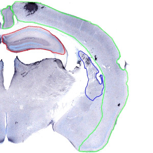
Overview image, showing the outline of regions of interest on the right half of a coronal brain section. Green: Cerebral Cortex, Red: Striatum, Blue: Hippocampus.
#10033
Huntington’s disease (HD) is a progressive neurodegenerative genetic disorder, caused by an autosomal dominant mutation on the Huntingtin gene (HTT). The mutation of HTT means that the length of a repeated section of the gene exceeds a normal range, resulting in an abnormal long poly-glutamine repeat on one part of the protein, causing the proteins to create hydrogen bonds and to form protein aggregates. The presence of the mutant proteins results in gradual damage to specific areas of the brain but the exact way this happens is not fully understood. The pathologic changes in the brain of HD patients affect muscle coordination and leads to cognitive decline, dementia and psychiatric problems. HD is also the most common genetic cause of chorea which is abnormal involuntary writhing movements.
Research into the mechanism of HD is primarily focused on the brain pathology the disease produces. Modeling the disease in animal models is critical for understanding the fundamental mechanisms of the disease and for supporting the early stages of drug development. The size and amount of the aggregates combined with the large area of the ROIs (Cerebral Cortex, Striatum, and Hippocampus) has previously made quantification very difficult.
By using digital image analysis based on virtual slides to quantify the presence of protein aggregates for evaluating e.g. effect of a drug in HD treatment studies, it is possible to obtain high-throughput quantification of aggregates without compromising the accuracy and quality of the results.
Overview image, showing the outline of regions of interest on the right half of a coronal brain section. Green: Cerebral Cortex, Red: Striatum, Blue: Hippocampus.
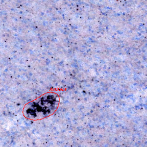
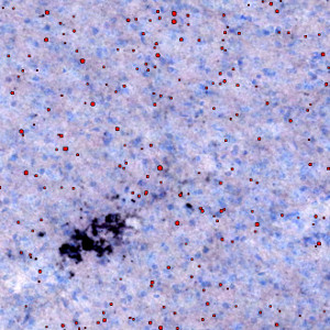
Examples of artifacts that will automatically be excluded by the image analysis protocol. The black spots in the image that are not annotated here as artifacts (red outline) will all count as true aggregates and will be included.
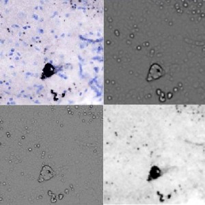
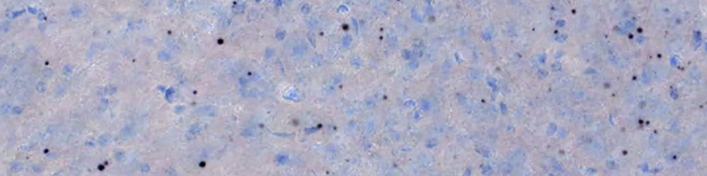
Illustration of the feature images created during pre-processing for use in the classification. From top left to bottom right the images represent: 1) Original image of area from Hippocampus. 2) Poly. Blob filter to enhance large aggregates. 3) Poly. Blob filter to enhance small aggregates. 4) Mean filter of blue color channel to allow for detection of artifacts.
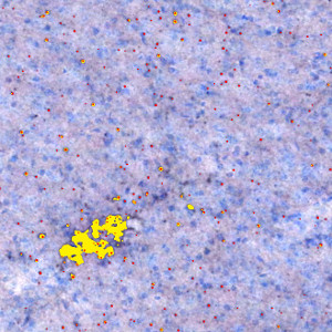
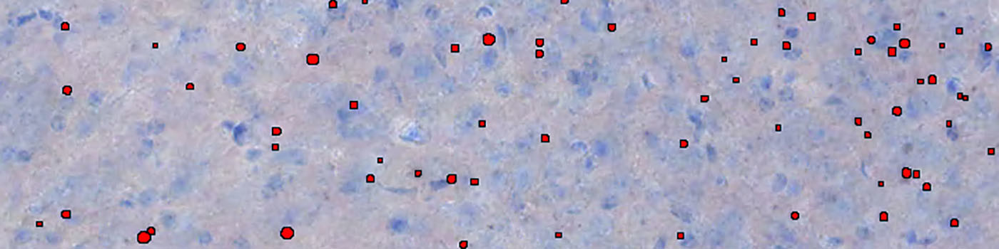
The result of the initial classification identifying aggregates and artifacts.
ARRAYIMAGER GRID CONFIGURATION
Arrayimager grid configuration: By using the Arrayimager™ a grid can be fitted on each slide to obtain a separate high magnification image for each hemisphere while uniquely identifying each hemisphere section with a Donor ID as well as core coordinates. This way each brain/hemisphere can easily be tracked during result reporting.
Quantitative Output variables
The output variables obtained from this protocol include:
Cortex Dist, Striatum Dist and Hippocampus Dist.: Aggregate area distribution
#Aggregate Cortex, #Aggregate Striatum and #Aggregate Hippocampus: Number of aggregates within each ROI.
Area Fraction Cortex, Area Fraction Striatum and Area Fraction Hippocampus: Percentage area occupied by aggregates per ROI per animal.
Methods
The right and left hemisphere of each brain must first be extracted as individual images by using the auxiliary APP for Arrayimager, to allow you to report the results per animal. When the images from each hemisphere have been extracted, the ROIs must be outlined manually as shown in FIGURE 1. Finally the APP for quantification can be applied.
The mutant Htt aggregates have a set of very distinct characteristics and can be classified based on their properties of shape, size and color. The aggregates appear distinct and are readily identified as compared to the artifacts observed in some sections. Representatives of the Htt aggregates versus artifacts are depicted in FIGURE 2.
In pre-processing, the Polynomial Blob filter is applied to enhance the aggregates. The diameter of the aggregates that we would like to include varies and for this reason, two Polynomial Blob filters of different size are applied. Both are used on the blue color band (RGB-B). Furthermore, a third feature image is applied to identify dark artifact areas. The feature images are illustrated in FIGURE 3.
Since the preprocessing steps will make the aggregates stand out as bright signals on a dark background, a threshold classifier will be sufficient to identify the aggregate class. The value of the threshold for each feature image is fine-tuned by examining a set of images that are representative for the entire dataset. See FIGURE 4 for an example of the classification before post processing.
Finally, a series of post processing steps is included, where the detected aggregates are evaluated on size (classified object that are too large or too small is discarded), shape (aggregates are evaluated based on the irregularity, i.e. how circular it is), and position relative to artifacts. The final result of the segmentation after post processing is shown in FIGURE 5.
Keywords
Huntington’s, protein aggregate, Striatum, Cerebral Cortex, Hippocampus, Htt, IHC, quantitative, digital pathology, image analysis.